Cumulative distribution function
In probability theory and statistics, the cumulative distribution function (CDF), or just distribution function, describes the probability that a real-valued random variable X with a given probability distribution will be found at a value less than or equal to x. Intuitively, it is the "area so far" function of the probability distribution. Cumulative distribution functions are also used to specify the distribution of multivariate random variables.
Contents |
Definition
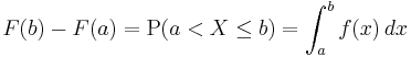
For every real number x, the cumulative distribution function of a real-valued random variable X is given by
where the right-hand side represents the probability that the random variable X takes on a value less than or equal to x. The probability that X lies in the interval (a, b], where a < b, is therefore

Here the notation (a, b], indicates a semi-closed interval.
If treating several random variables X, Y, ... etc. the corresponding letters are used as subscripts while, if treating only one, the subscript is omitted. It is conventional to use a capital F for a cumulative distribution function, in contrast to the lower-case f used for probability density functions and probability mass functions. This applies when discussing general distributions: some specific distributions have their own conventional notation, for example the normal distribution.
The CDF of a continuous random variable X can be defined in terms of its probability density function ƒ as follows:
Note that in the definition above, the "less than or equal to" sign, "≤", is a convention, not a universally used one (e.g. Hungarian literature uses "<"), but is important for discrete distributions. The proper use of tables of the binomial and Poisson distributions depend upon this convention. Moreover, important formulas like Levy's inversion formula for the characteristic function also rely on the "less or equal" formulation.
In the case of a random variable X which has distribution having a discrete component at a value x0,

where F(x-) denotes the limit from the left of F at x0: i.e. lim F(y) as y increases towards x0.
Properties
Every cumulative distribution function F is (not necessarily strictly) monotone non-decreasing (see monotone increasing) and right-continuous.Furthermore,
Every function with these four properties is a CDF. The properties imply that all CDFs are càdlàg functions.
If X is a purely discrete random variable, then it attains values x1, x2, ... with probability pi = P(xi), and the CDF of X will be discontinuous at the points xi and constant in between:
If the CDF F of X is continuous, then X is a continuous random variable; if furthermore F is absolutely continuous, then there exists a Lebesgue-integrable function f(x) such that
for all real numbers a and b. (The first of the two equalities displayed above would not be correct in general if we had not said that the distribution is continuous. Continuity of the distribution implies that P (X = a) = P (X = b) = 0, so the difference between "<" and "≤" ceases to be important in this context.) The function f is equal to the derivative of F almost everywhere, and it is called the probability density function of the distribution of X.
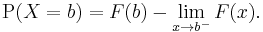
Point probability
The "point probability" that X is exactly b can be found as
Kolmogorov–Smirnov and Kuiper's tests
The Kolmogorov–Smirnov test is based on cumulative distribution functions and can be used to test to see whether two empirical distributions are different or whether an empirical distribution is different from an ideal distribution. The closely related Kuiper's test is useful if the domain of the distribution is cyclic as in day of the week. For instance we might use Kuiper's test to see if the number of tornadoes varies during the year or if sales of a product vary by day of the week or day of the month.
Complementary cumulative distribution function (tail distribution)
Sometimes, it is useful to study the opposite question and ask how often the random variable is above a particular level. This is called the complementary cumulative distribution function (ccdf) or simply the tail distribution or exceedance, and is defined as

This has applications in statistical hypothesis testing, for example, because one-sided P-value is the probability of observing a test statistic at least as extreme as the one observed; hence, the one-sided P-value is simply given by the ccdf.
In survival analysis,  is called the survival function and denoted
  , while the term reliability function is common in engineering.
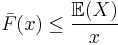
Properties
- For a non-negative random variable having an expectation, Markov's inequality states that:
- As
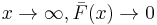 , and in fact
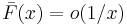
Proof: Assuming X has density function f, we have for any 
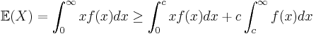
Recognizing 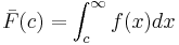 and rearranging terms:
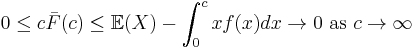
as claimed.
Folded cumulative distribution
While the plot of a cumulative distribution often has an S-like shape, an alternative illustration is the folded cumulative distribution or mountain plot, which folds the top half of the graph over,[1][2] thus using two scales, one for the upslope and another for the downslope. This form of illustration emphasises the median and dispersion of the distribution or of the empirical results.
Examples
As an example, suppose X is uniformly distributed on the unit interval [0, 1]. Then the CDF of X is given by
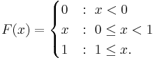
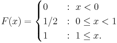
Suppose instead that X takes only the discrete values 0 and 1, with equal probability. Then the CDF of X is given by
Inverse distribution function (quantile function)
If the CDF F is strictly increasing and continuous then ![F^{-1}( y ), y \in [0,1]](/2012-wikipedia_en_all_nopic_01_2012/I/0a97cbe5a0c0b47d058c4492467472c3.png) is the unique real number
is the unique real number  such that
  .
.
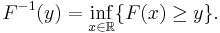
Unfortunately, the distribution does not, in general, have an inverse. One may define, for ![y \in [0,1]](/2012-wikipedia_en_all_nopic_01_2012/I/ab3abad183cd9e117cb5711a60e1bc1d.png) , the generalized inverse distribution function:
, the generalized inverse distribution function:
- Example 1: The median is
 .
. - Example 2: Put
 . Then we call
  the 95th percentile.
The inverse of the cdf is called the quantile function.
The inverse of the cdf can be used to translate results obtained for the uniform distribution to other distributions. Some useful properties of the inverse cdf are:
 is nondecreasing
 if and only if
- If
 has a
has a ![U[0, 1]](/2012-wikipedia_en_all_nopic_01_2012/I/96a9c75abd000127ef1098bcd27eb72c.png) distribution then
distribution then  is distributed as
  . This is used in random number generation using the inverse transform sampling-method.
 - If
 is a collection of independent -distributed random variables defined on the same sample space, then there exist random variables
  such that is distributed as and
  with probability 1 for all
  .
.
Multivariate case
When dealing simultaneously with more than one random variable the joint cumulative distribution function can also be defined. For example, for a pair of random variables X,Y, the joint CDF is given by

where the right-hand side represents the probability that the random variable X takes on a value less than or equal to x and that Y takes on a value less than or equal to y.
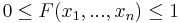
Every multivariate CDF is:
- Monotonically non-decreasing for each of its variables
- Right-continuous for each of its variables.
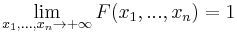 and
and 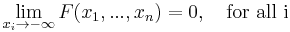
See also
- Descriptive statistics
- Empirical distribution function
- Cumulative frequency analysis
- Q-Q plot
- Ogive
- Single crossing condition
References
- ^ Gentle, J.E. (2009). Computational Statistics. Springer. http://books.google.de/books?id=m4r-KVxpLsAC&lpg=PA348&ots=8Wxj0G_GC6&dq=folded%20cumulative%20distribution%20or%20mountain%20plot&hl=en&pg=PA348#v=onepage&q=folded%20cumulative%20distribution%20or%20mountain%20plot&f=false. Retrieved 2010-08-06.
- ^ Monti, K.L. (1995). "Folded Empirical Distribution Function Curves (Mountain Plots)". The American Statistician 49: 342–345. JSTOR 2684570.
|
|||||||||||||